Flat-field
Quickstart
The command for running the flat-field procedure is called by:
pylongslit_flat PATH_TO_CONFIG_FILE
The flat-field procedure produces a master flat-field frame master_flat.fits,
and places it in the output directory specified in the configuration file. The master
flat is a median-combined, spectrally, and (optionally) spatially normalized flat-field frame.
It holds the information about the pixel-to-pixel sensitivity of the detector, where
pixel value 1.0 is the mean pixel intensity for the detector.
The flat-field procedure has several stages - all described individually below in this documentation. The stages are:
Median combination of the raw flat frames.
Spectral normalization of the master flat.
(Optional) Spatial normalization of the master flat.
The raw flat frames are read from the directory specified in the configuration file
under the parameter "flat_dir". Make sure that no other file types are present in the
directory.
Median combination of the raw flat frames
The raw flat frames get median combined the same way as described in the
bias procedure. The difference is that the flat frames are
first bias-subtracted and if the detector has a significant dark current,
the dark current can also be removed. Similar to the bias procedure,
the user can decide whether bootstrapping is necessary for the error estimation
of the median by setting the parameter "bootstrap_errors" to true
or false in the configuration file. To see a full description of the
error estimation in the software, please refer to the description of uncertainty calculations.
Spectral normalization of the master flat
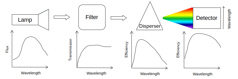
Before the light from the flat-field illumination source (such as a halogen lamp) reaches the detector, it has to pass through an array of optical elements - such as dispersers and filters. These optical elements, and the detector itself, have wavelength-dependent efficiencies. Because of the disperser, photons with different wavelengths will hit the detector in different places, meaning that these wavelength-dependent efficiencies will make the flat-field non-uniform in the spectral direction, as sketched below:
In this step, we want to normalize this spectral response, as we are only interested in the pixel-to-pixel sensitivity of the detector when flat-fielding.
First, a slice-spectrum is taken from the median flat in the spectral direction.
This is analogous to the arc lamp 1d spectrum extraction in the wavelength calibration. The "offset_middle_cut" and "pixel_cut_extension" from the wavelength calibration
parameters can be used to adjust the shape and position of the slice-spectrum
(see the documentation for line reidentification).
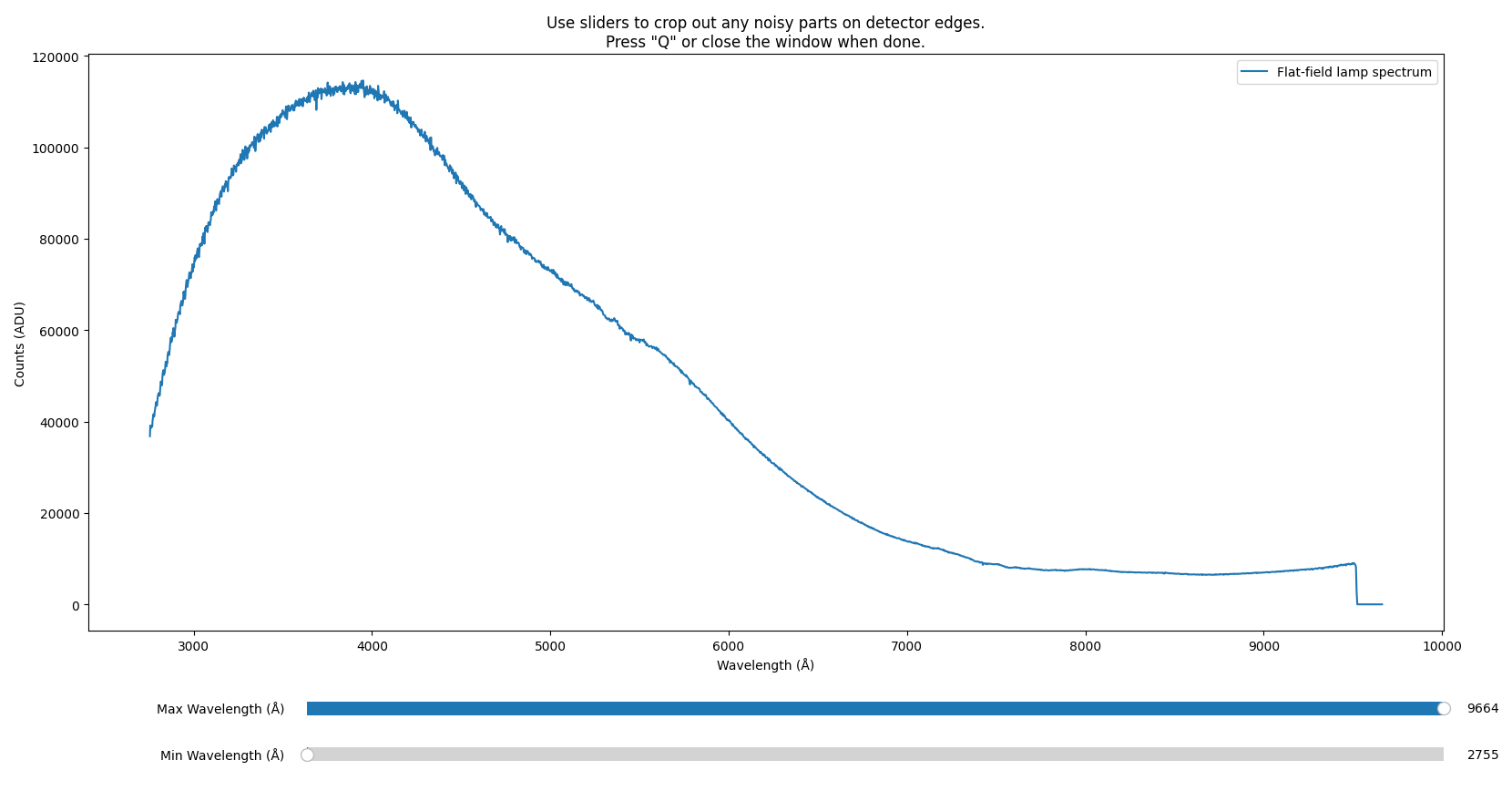
Further, you will have the option to manually crop away any noisy edges that
would corrupt later fitting (in the example below from the SDSS_J213510+2728
tutorial data, this would be the overscan region with zero counts):
A B-Spline is then fitted to the slice-spectrum (wavelength vs. counts) to estimate the spectral response of the detector:
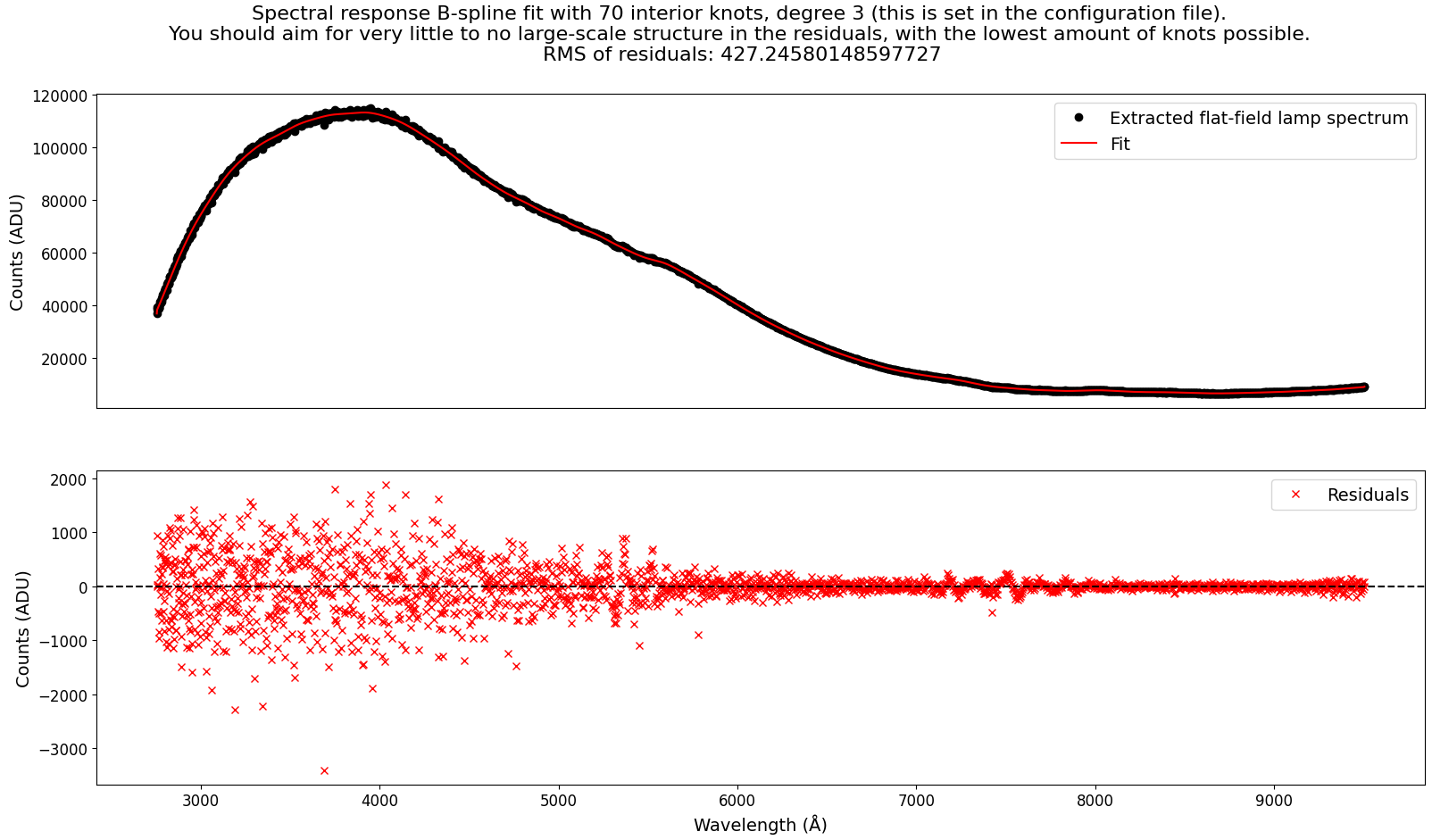
Here, the main thing to watch out for is overfitting. The B-Spline should be a smooth representation of the spectral response, and should not be overfitting to the level of pixel-to-pixel deviations. The following parameters can be adjusted to control the fitting, with example values:
"flat": {
    "knots_spectral_bspline": 70, # number of bspline knots
    "degree_spectral_bspline": 3 # degree of the bspline
}
The fitted 1d spectral response model is then evaluated at each pixel on the detector in order to construct a 2d spectral response model. The median flat is then divided by this 2d spectral response model to produce the spectrally normalized master flat.
(Optional) Spatial normalization of the master flat
The same way that the flat-field is non-uniform in the spectral direction,
so might it be in the spatial direction, if the illumination source is not
uniform in the spatial direction. In this case, you can also normalize the
master flat in the spatial direction. This is done by setting the parameter
"skip_spacial" to false in the configuration file. Whether it is necessary/suitable
to do is discussed below.
The spatial normalization procedure is very similar to the spectral normalization. First, a slice-spectrum is taken from the median flat in the spatial direction, and you can crop away any noisy edges. In the case for the tutorial data GQ1218+0832, the edges with no signal should be cropped away:
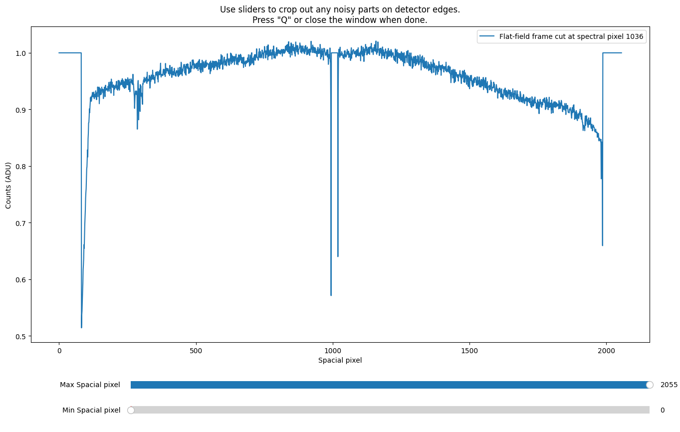
The gap in the middle of the GTC Osiris detector mosaic is also unwanted, but the software does some sigma-clipping to remove outliers, so the fits should be fine if your own data has similar artifacts.
A B-Spline is then fitted to every spatial column of the detector, and a sample is taken for quality assessment:
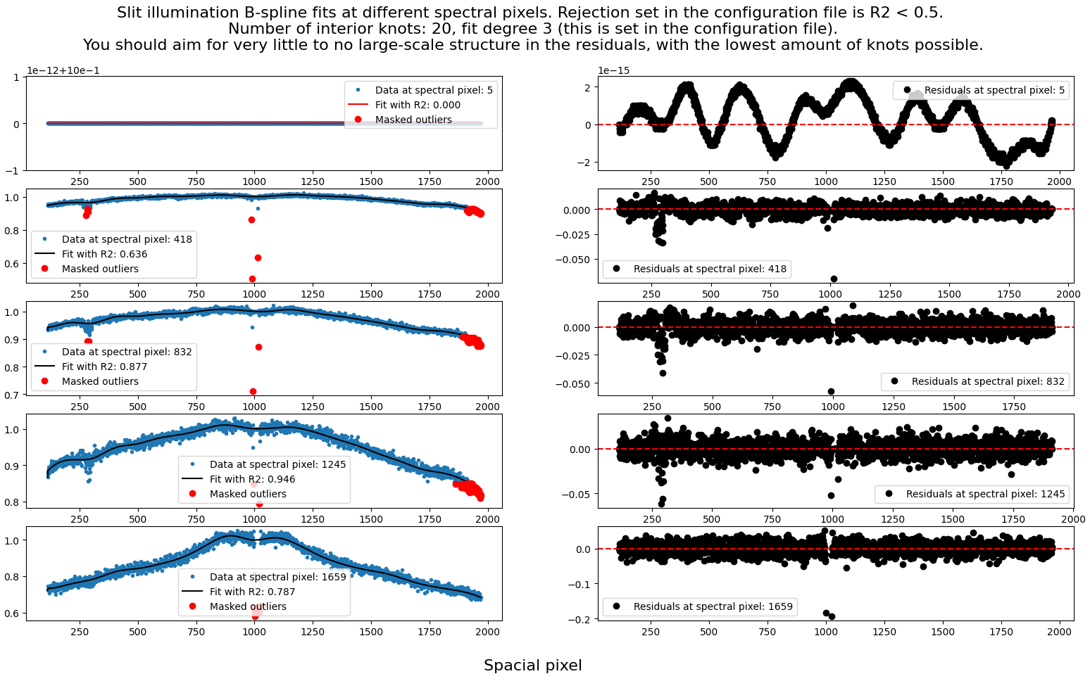
As with the spectral normalization, the main thing to watch out for is overfitting. The B-Spline should be a smooth representation of the spatial response, and should not be overfitting to the level of pixel-to-pixel deviations. Furthermore, since there are many fits, they are rejected/accepted automatically based on a user-defined \(R^2\) threshold (ex. the first fit in the above figure is automatically rejected). The following parameters can be adjusted to control the fitting (with example values):
"flat": {
    "knots_spacial_bspline": 4, # number of bspline knots
    "degree_spacial_bspline": 3, # degree of the bspline
    "R2_spacial_bspline": 0.4 # R^2 threshold for the fits
}
From experience, the \(R^2\) threshold might need to be set relatively low, as the fits can be quite noisy.
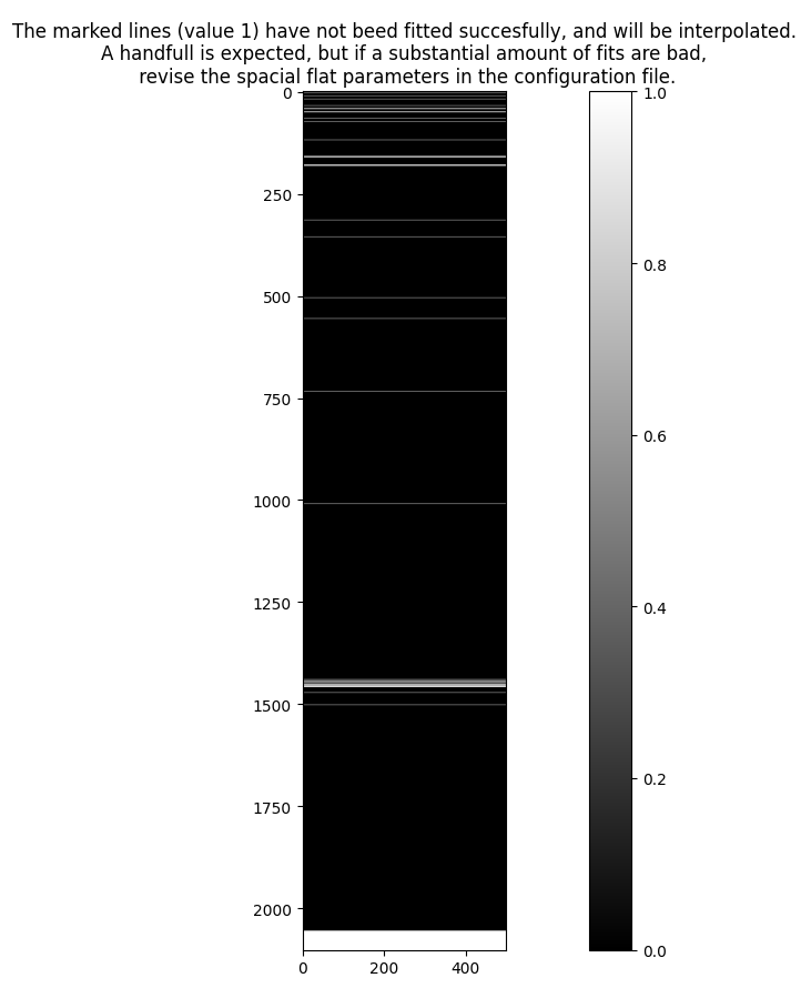
The spatial model is constructed as a stack of the individual 1d fits. For the fits that failed, the model is interpolated from the nearest successful fits. The number of failed fits is plotted on the detector for quality assessment.
As shown with the example dataset SDSS_J213510+2728, it is okay to see some failed fits scattered around the detector and in the edges, but you should revise the parameters if large areas (that are not detector edges) fail:
Final Quality Assessment Plot
Upon exiting, the software will produce a plot that shows the master flat and a histogram of the pixel values through each stage of the flat-fielding:
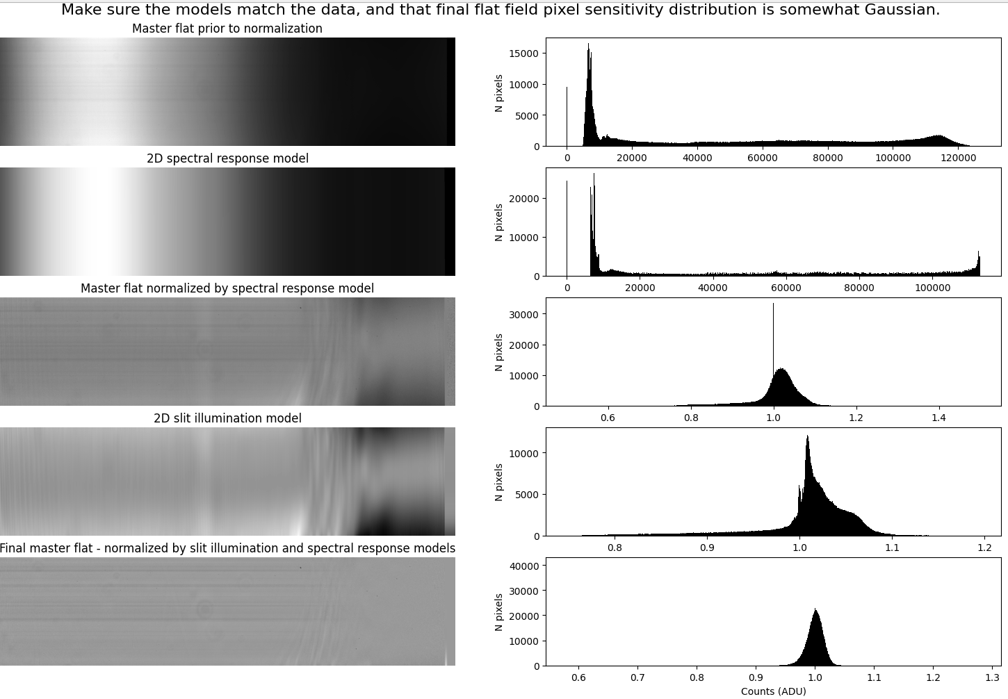
The final master flat should be mostly uniform, with an approximately Gaussian distribution of pixel values. Non-uniformities in the flat-field are usually caused by dust on the optics, and not only is it okay if you see them in the master flat, it is exactly what you are looking for - as these will now get normalized when dividing the observations with the master flat:
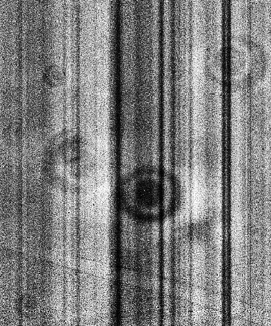
The stripes seen in the SDSS_J213510+2728 tutorial data are inherited from the raw frames and are not caused by the flat-fielding procedure, but by dust flakes on the entrance slit, also visible on a raw (non-normalized) spectral flat image:

Considerations on spatial normalization
The software can optionally normalize the flat-field in the spatial direction (this option is set in the configuration file). This operation assumes that any large-scale variation along the slit in a dome or internal flat is caused by the flat-field illumination source itself (for example, an uneven lamp). Under that assumption, dividing by the spatial profile of the flat removes the illumination pattern of the lamp while preserving the true detector and pixel response.
However, this assumption is not always valid. The telescope and instrument optics can also imprint a position-dependent throughput along the slit. This instrumental response is present in science exposures, but it may not be reproduced by the internal/dome-flat illumination. As a result, the spatial profile of an internal/dome flat may not match the true slit illumination seen in on-sky frames. In such cases, applying spatial normalization based on the internal/dome flat can introduce incorrect corrections in the reduced data.
Because of this, spatial normalization is optional and may not be appropriate for all instruments.
You can try to do a reduction run with spatial normalization, and if you start seeing strange artifacts in the reduced science frames, you can try to do the reduction without spatial normalization.
For users new to data reduction - short introduction to flat-fielding
Since the number of pixels on a detector is in the order of millions, it is necessary to assume homogeneous pixel sensitivity throughout the detector in order to make any further computations feasible. In other words, we want to assume that any registered photon on the detector will be registered with the same efficiency regardless of what pixel registers it. The physical properties of CCD detectors do not verify this assumption, but this can be reached through calibration.
Theoretically, the flat-field calibration procedure requires exposing the detector with completely uniform light throughout the detector. Since every pixel receives the same amount of light, any differences in registered counts between pixels can be used to evaluate the difference in pixel-to-pixel sensitivity. This kind of exposure of uniform light is called a flat-field. In practice, the procedure for flat-fielding the detector while performing spectroscopy is more complicated, as it requires a substantial amount of modelling and removing of any other sensitivity variations that are not pixel-to-pixel - such as wavelength-dependent sensitivity and spatial illumination patterns. From personal experience, the flat-fielding procedure is the most controversial step in spectroscopic data reduction, as the ideological assumption of uniform illumination is practically impossible to achieve.
Wavelength Calibration ← Previous pipeline step
Next pipeline step → Raw frame reduction