Identify arc lines
In this step, we manually identify the lines in the arc-lamp spectrum, by cross-referencing with a known calibrated line spectrum.
For this step we use an application originally developed by Jens-Kristian Krogager for the PyNOT software.
This step is by far the most time-consuming for the user, as a fair amount of user work is needed. Expect this to be challenging at first, if you have not tried this type of routine before. Feel free to re-use the already made tables.
For this procedure, you will need to acquire a calibrated arc lamp spectrum for your instrument (these will also differ for every different disperser used for the same instrument). For this tutorial, we are using NOT ALFOSC disperser grating #4, and an arc spectrum composed of helium and neon lines, taken from: https://www.not.iac.es/instruments/alfosc/lamps/. Furthermore, you will need a line-list with two columns, the first being the wavelength of the line in Angstroms, and the second being the element of the line. For the HeNe lamp used in the tutorial, the beginning of the list looks like this:
3614.671653955192 HeI
3706.05727477696 HeI
3889.7479741029447 HeI
3965.8488118806977 HeI
4027.32686731872 HeI
4121.974633218378 HeI
You can see the full list at https://github.com/KostasValeckas/PyLongslit_dev/blob/main/database/line_lists/alfosc_he_ne_vac.dat.
This line list is taken from the same link as the arc lamp maps, and converted from air to vacuum line wavelengths. As a user you can decide yourself whether to use the air or vacuum line, just know that your end product will also be in the same system.
The application is called by:
pylongslit_identify_arcs PATH_TO_CONFIG_FILE
When the command is executed, a GUI/interactive plot window will open.
A 1d-spectrum cut will be taken from the master_arc.fits file produced
in the previous step, and displayed in the window. You
then have to manually load the above described line list by clicking on the
Load LineList button in the upper left corner. When this is done, for the
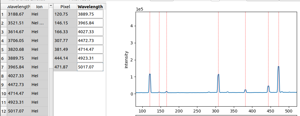
example dataset SDSS_J213510+2728, the window should look like this:
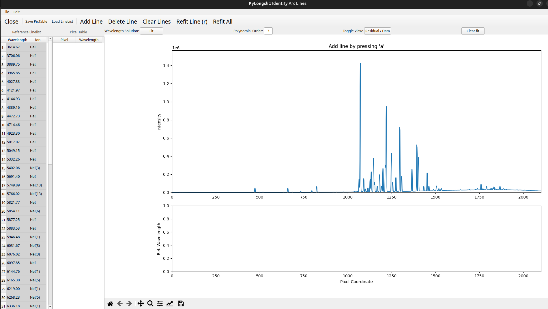
Identifying the lines
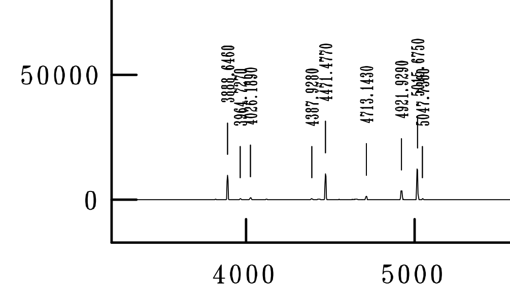
Now, you have to use the reference spectra (also called the arc maps) to identify the wavelengths of the lines in the arc spectrum. This is done by clicking on the Add Line button, and then clicking on the arc spectrum where you think a line is, and then manually typing in the wavelength of the line. Below is an example for a small Helium portion of the spectrum, with a zoom in of the corresponding reference spectrum, taken from https://www.not.iac.es/instruments/alfosc/lamps/map-g04-he-1.pdf:
Here there is a small offset between the reference spectrum (lowest picture) and the line list (upper left corner) - this is because we use vacuum wavelengths, while the reference spectrum is in air.
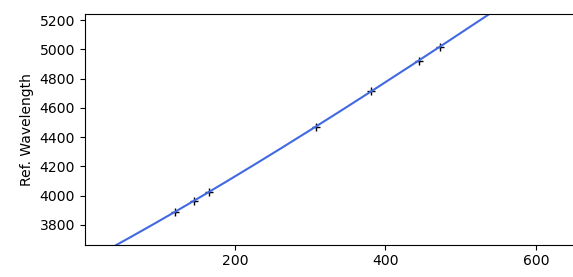
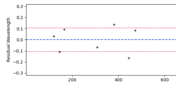
After you have found a handful of lines, you can click on the Fit button to make a polynomial fit for a function that describes wavelength as a function of pixel. You can use the Residual/Data button to change displays between the fit curve and the residuals of the fit in order to evaluate the fit quality. For the small amount of lines shown above, this looks like this:
When you have obtained a fit, and try to Add Line again, the program will now use the fit to extrapolate the wavelength of the line you are trying to add, and look for it in the line list. If it finds a match, it will automatically add it. If it does not find a match, it will show a message indicating so, but it will still add the line - you will then have to correct it manually. If your fit does not seem to be good, you can click on the Clear fit button to remove it, and then add more lines manually, or change the polynomial order. You can also selectively remove one or all lines.
From here on, you have to (correctly) identify as many lines as possible by iterating through this process:
Add lines manually
Fit
Use the fit to add more lines
Refit - correct outliers - come back to 1. or 2. and repeat until you are satisfied with the results.
Note
The end products of the pipeline will depend highly on the quality of the line identification. The wavelength calibration routine will use the identified lines to refine the line centers and trace the lines through the whole detector - but it cannot find new lines if they have not been manually identified. The line identification puts an upper boundary on how well the wavelength calibration routine can perform. Even though this step is by far the most time-consuming, it should not be rushed. However, you will very likely be unable to identify all lines, and the ones that cause uncertainty should be left out. Try to identify lines in all parts of the spectrum.
Saving the line list: When you are satisfied with the identification, you need to save the pixel table (the pixel vs. wavelength table). Press File -> Save PixTable and save the file.
Note
For the tutorials of SDSS_J213510+2728 and GQ1218+0832 , we have already identified the lines, so you have a starting point to work with. You can inspect the files by pressing File -> Load PixTable. To proceed in the tutorial, you can either try to improve our fit, or move on directly using it. All current identified lines for different instruments and their configurations can be found here.
Parameter options
The relevant parameters for the identify procedure are (with example values):
"wavecalib" : {
   "offset_middle_cut": 0,
   "pixel_cut_extension": 2,
   "center_guess_pixtable": "/home/kostas/Documents/PyLongslit_dev/database/pixtables/alfosc_grating4_hene_pixtable.dat",
},
The GUI takes a 1d-spectrum from the master_arc.fits file. It takes the
spectrum from the middle of the image. Sometimes, the middle of the image is not the best
place, so the offset_middle_cut parameter can be used to offset the cut from the middle
by a certain amount of pixels.
The pixel_cut_extension parameter is used to decide how many detector rows to use for the
1d-spectrum cut. If pixel_cut_extension is set to 0, only one row will be used. If it is set to 2,
the middle row +/- 2 rows will be used and then averaged and so forth. This is useful if the arc line spectrum
is noisy, as averaging removes some of the noise. However, the cut should not be wider than necessary, as the line centers change gradually
in the spatial direction (see description of line tilts).
When you are done, you have to link the path to the pixel table to the
center_guess_pixtable parameter, as the wavelength calibration routine will need it.
Combining arc frames ← Previous pipeline step
Next pipeline step → Wavelength Calibration
